Self-Explaining Neural Networks: A Review

For many applications, understanding why a predictive model makes a certain prediction can be of crucial importance. In the paper “Towards Robust Interpretability with Self-Explaining Neural Networks”, David Alvarez-Melis and Tommi Jaakkola propose a neural network model that takes interpretability of predictions into account by design. In this post, we will look at how this model works, how reproducible the paper’s results are, and how the framework can be extended.

First, a bit of context. This blog post is a by-product of a student project that was done with a group of 4 AI grad students: Aman Hussain, Chris Hoenes, Ivan Bardarov, and me. The goal of the project was to find out how reproducible the results of the aforementioned paper are, and what ideas could be extended. To do this, we re-implemented the framework from scratch. We have released this implementation as a package here. In general, we find that the explanations generated by the framework are not very interpretable. However, the authors provide several valuable ideas, which we use to propose and evaluate several improvements.

Before we dive into the nitty gritty details of the model, let’s talk about why we care about explaining our predictions in the first place.

Transparency in AI

As ML systems become more omnipresent in societal applications such as banking and healthcare, it’s crucial that they should satisfy some important criteria such as safety, not discriminating against certain groups, and being able to provide the right to explanation of algorithmic decisions. The last criterion is enforced by data policies such as the GDPR, which say that people subject to the decisions of algorithms have a right to explanations of these algorithms.

These criteria are often hard to quantify. Instead, a proxy notion is regularly made use of: interpretability. The idea is that if we can explain why a model is making the predictions it does, we can check whether that reasoning is reliable. Currently, there is not much agreement on what the definition of interpretability should be or how to evaluate it.

Much recent work has focused on interpretability methods that try to understand a model’s inner workings after it has been trained. Well known examples are LIME and SHAP. Most of these methods make no assumptions about the model to be explained, and instead treat them like a black box. This means they can be used on any predictive model.

Another approach is to design models that are transparent by design. This approach is also taken by Alvarez-Melis and Jaakkola, who I will be referring to as ‘‘the authors’’ from now on. They propose a self-explaining neural network (SENN) that optimises for transparency during the learning process, (hopefully) without sacrificing too much modeling power.

Self Explaining Neural Networks (SENN)

Before we design a model that generates explanations, we must first think about what properties we want these explanations to have. The authors suggest that explanations should have the following properties:

• Explicitness: The explanations should be immediate and understandable.
• Faithfulness: Importance scores assigned to features should be indicative of “true” importance.
• Stability: Similar examples should yield similar explanations.

Linearity

The authors start out with a linear regression model and generalize from there. The plan is to generalize the linear model by allowing it to be more complex, while retaining the interpretable properties of a linear model. This approach is motivated by arguing that a linear model is inherently interpretable. Despite this claim’s enduring popularity, it is not always entirely valid¹. Regardless, we continue with the linear model.

Say we have input features \(x_1, \dots, x_n\) and parameters \(\theta_1, \dots, \theta_n\). The linear model (omitting bias for clarity) returns the following prediction: \(f(x) = \sum_{i}^{k} \theta_i x_{i}.\)

Basis Concepts

The first step towards interpretability is taken by first computing interpretable feature representations \(h(x)\) of the input \(x\), which are called basis concepts (or concepts). Instead of acting on the input directly, the model acts on these basis concepts: \(f(x) = \sum_{i}^{k} \theta_i h(x)_{i}.\)

We see that the final prediction is some linear combination of interpretable concepts. The \(\theta_i\) can now be interpreted as importance or relevance scores for a certain concept \(h(x)_i\).

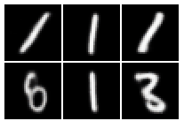
Say we are given an image \(x\) of a digit and we want to detect which digit it is. Then each concept \(h(x)_i\) might for instance encode stroke width, global orientation, position, roundness, and so on.

Concepts like this could be generated by domain experts, but this is expensive and in many cases infeasible. An alternative approach is to learn the concepts directly. It cannot be stressed enough that the interpretability of the whole framework depends on how interpretable the concepts are. Therefore, the authors propose three properties concepts should have and how to enforce them:

1. Fidelity: The representation of \(x\) in terms of concepts should preserve relevant information.

   This is enforced by learning the concepts \(h(x)\) as the latent encoding of an autoencoder. An autoencoder is a neural network that learns to map an input \(x\) to itself by first encoding it into a lower dimensional representation with an encoder network \(h\) and then creating a reconstruction \(\hat{x}\) with a decoder network \(h_\mathrm{dec}\), i.e. \(\hat{x} = h_\mathrm{dec}(h(x))\). The lower dimensional representation \(h(x)\), which we call its latent representation, is a vector in a space we call the latent space. It therefore needs to capture the most important information contained in \(x\). This can be thought of as a nonlinear version of PCA.

2. Diversity: Inputs should be representable with few non-overlapping concepts.

   This is enforced by making the autoencoder mentioned above sparse. A sparse autoencoder is one in which only a relatively small subset of the latent dimensions activate for any given input. While this indeed forces an input to be representable with few concepts, it does not really guarantee that they should be non-overlapping.

3. Grounding: Concepts should have an immediate human-understandable interpretation.

   This is a more subjective criterion. The authors aim to do this by providing interpretations for concepts by prototyping. For image data, they find a set of observations that maximally activate a certain concept and use those as the representation for that concept. While this may seem reasonable at first, we will see later that this approach is quite problematic.

As mentioned above, the approaches taken by the authors to achieve diversity and grounding have quite some problems. The extension that we introduce aims to mitigate these.

Keeping it Linear

In the last section, we introduced basis concepts. However, the model is still too simple, since the relevance scores \(\theta_i\) are fixed. We therefore make the next generalization: the relevance scores are now also a function of the input. This leads us to the final model²:

\[f(x) = \sum_{i}^{k} \theta(x)_i h(x)_{i}.\]

To make the model sufficiently complex, the function computing relevance scores \(\theta\) is actualized by a neural network. A problem with neural networks, however, is that they are not very stable. A small change to the input may lead to a large change in relevance scores. This goes against the stability criterion for explanations introduced earlier. To combat this, the authors propose to make \(\theta\) behave linearly in local regions, while still being sufficiently complex globally. This means that a small change in \(h\) should lead to only a small change in \(\theta\). To do this, they add a regularization term, which we call the robustness loss³, to the loss function.

In a classification setting with multiple classes, relevance scores \(\theta\) are estimated for each class separately. An explanation is then given by the concepts and their corresponding relevance scores⁴. The figure below shows an example of such an explanation.

The authors interpret such an explanation in the following way. Looking at the first input, a “9”, we see that concept 3 has a positive contribution to the prediction that it is a 9. Concept 3 seems to represent a horizontal dash together with a diagonal stroke, which seems to be present in the image of a 9. As you may have noticed, these explanations also require some imagination.

Implementation

Although a public implementation of SENN is available, the authors have not officially released that code with the paper. There also seems to be a major bug in this code. Therefore, we re-implement the framework with the original paper as ground truth.

On a high level, the SENN model consists of three main building blocks: a parameterizer \(\theta\), a conceptizer \(h\), and an aggregator \(g\), which is just the sum function in this case. The parameterizer is actualized by a neural network, and the conceptizer is actualized by an autoencoder. The specific implementations of these networks may vary. For tabular data, we may use fully connected networks and for image data, we may use convolutional networks. Here is an overview of the model:

To train the model, the following loss function is minimized:

\[\begin{align} \mathcal{L} := \mathcal{L}_y(f(x), y) + \lambda \mathcal{L}_\theta(f(x)) + \xi \mathcal{L}_h(x), \label{eq:total_loss} \end{align}\]

where

• \(\mathcal{L}_y(f(x), y)\) is the classification loss, i.e. how well the model predicts the ground truth label.
• \(\mathcal{L}_\theta(f(x))\) is the robustness loss. \(\lambda\) is a regularization parameter controlling how heavily robustness is enforced.
• \(\mathcal{L}_h(x)\) is the concept loss. The concept loss is a sum of 2 different losses: reconstruction loss and sparsity loss. \(\xi\) is a regularization parameter on the concept loss.

Reproducibility

If it is impossible to reproduce a paper’s results, it is hard to verify the validity of the obtained results. Even if the results are valid, it will be hard to build upon that work. Reproducibility has therefore recently been an important topic in many scientific disciplines. In AI research, there have been initiatives to move towards more reproducible research. NeurIPS, one of the biggest conferences in AI, introduced a reproducibility checklist last year. Although it is not mandatory, it is a step in the right direction.

Results

The main goal of our project was to reproduce a subset of the results presented by the authors. We find that while we are able to reproduce some results, we are not able to reproduce all of them.

In particular, we are able to achieve similar test accuracies on the Compas and MNIST datasets, a tabular and image dataset respectively, which seems to validate the authors’ claim that SENN models have high modelling capacity. Even though this is the case, the MNIST and Compas datasets are of low complexity. The relatively high performance on these datasets is therefore not sufficient to show that SENN models are on par with non-explaining state-of-the-art models.

We also look at the trade off between robustness of explanations and model performance. We see that enforcing robustness more decreases classification accuracy. This behavior matches up with the authors’ findings. However, we find the accuracy drop for increasing regularization to be significantly larger than reported by the authors.

Assessing the quality of explanations is inherently subjective. It is therefore difficult to link the quality of explanations to reproducibility. However, we can still partially judge reproducibility by qualitative analysis. In general, we see that finding an example whose explanation “makes sense” is difficult and that such an example is not representative of the generated examples. Therefore, we conclude that obtaining good explanations is, in that sense, not reproducible.

Interpretation

How do we interpret this failure to reproduce? Although it is tempting to say that the initial results are invalid, this might be too harsh and unfair. There are many factors that influence an experiment’s results. Although our results are discouraging, more experiments need to be done to have a better estimate of the validity of the framework. Even if this is the case, the authors provide a useful starting point for further research. We take a first step, which involves improving the learned concepts.

Disentangled SENN (DiSENN)

As we have seen, the current SENN framework hardly generates interpretable explanations. One important part of this is the way concepts are represented and learned. A single concept is represented by a set of data samples that maximizes that concept’s activation. The authors reason that we can read off what the concept represents by examining these samples. However, this approach is problematic.

Firstly, only showcasing the samples that maximize an encoder’s activation is quite arbitrary. One could just as well showcase samples that minimize the activation instead, or use any other method. These different approaches lead to different interpretations even if the learned concepts are the same. The authors also hypothesize that a sparse autoencoder will lead to diverse concepts. However, enforcing only a subset of dimensions to activate for an input does not explicitly enforce that these concepts should be non-overlapping. For digit recognition, one concept may for example represent both thickness and roundness at the same time. That is, each single concept may represent a mix of features that are entangled in some complex way. This greatly increases the complexity of interpreting any concept on its own. An image, for example, is formed from the complex interaction of light sources, object shapes, and their material properties. We call each of these component features a generative factor.

To enhance concept interpretability, we therefore propose to explicitly enforce disentangling the factors of variation in the data (generative factors) and using these as concepts instead. Different explanatory factors of the data tend to change independently of each other in the input distribution, and only a few at a time tend to change when one considers a sequence of consecutive real-world inputs. Matching a single generative factor to a single latent dimension allows for easier human interpretation⁵.

We enforce disentanglement by using a \(\beta\)-VAE, a variant of the Variational Autoencoder (VAE), to learn the concepts. If you are unfamiliar with VAEs, I suggest reading this blog post. Whereas a normal autoencoder maps an input to a single point in the latent space, a VAE maps an input to a distribution in the latent space. We want, and enforce, this latent distribution to look “nice” in some sense. A unit Gaussian distribution is generally the go-to choice for this. This is done by minimizing the KL-divergence between a Gaussian and the learned latent distribution.

\(\beta\)-VAE introduces a hyperparameter \(\beta\) that enables a heavier regularization on the latent distribution (i.e. higher KL-divergence penalty). The higher \(\beta\), the more the latent space will be encouraged to look like a unit Gaussian. Since the dimensions of a unit Gaussian are independent, these latent factors will be encouraged to be independent as well.

Each latent space dimension corresponds to a concept. Since interpolation in the latent space of a VAE can be done meaningfully, a concept can be represented by varying its corresponding dimension’s values and plugging it into the decoder⁶. It is easier to understand visually:

We see here that the first row represents the width of the number, while the second row represents a number’s angle. This figure is created by mapping an image to the latent space, changing one dimension in this latent space and then seeing what happens to the reconstruction.

We thus have a principled way to generate prototypes, since meaningful latent space traversal is an inherent property of VAEs. Another advantage is that prototypes are not constrained to the input domain. The prototypes generated by the DiSENN are more complete than highest activation prototypes, since they showcase a much larger portion of a concept dimension’s latent space. Seeing the transitions in concept space provides a more intuitive idea of what the concept means.

We call a disentangled SENN model with \(\beta\)-VAE as the conceptizer a DiSENN model. The following figure shows an overview of the DiSENN model. Only the conceptizer subnetwork has really changed.

We now examine the DiSENN explanations by analyzing a generated DiSENN explanation for the digit 7.

The contribution of concept \(i\) to the prediction of a class \(c\) is given by the product of the corresponding relevance and concept activation \(\theta_{ic} \cdot h_i\). First, we look at how the concept prototypes are interpreted. To see what a concept encodes, we observe the changes in the prototypes in the same row. Taking the second row as an example, we see a circular blob slowly disconnect at the left corner to form a 7, and then morph into a diagonal stroke. This explains the characteristic diagonal stroke of a 7 connected with the horizontal stroke at the right top corner but disconnected otherwise. As expected, this concept has a positive contribution to the prediction for the real class, digit 7, and a negative contribution to that of another incorrect class, digit 5.

However, despite the hope that disentanglement encourages diversity, we observe that concepts still demonstrate overlap. This can be seen from concepts 1 and 2 in the previous figure. This means that the concepts are still not disentangled enough, and the problem of interpretability, although alleviated, remains. The progress of good explanations using the DiSENN framework therefore depends on the progress of research in disentanglement.

What next?

In this post, we’ve talked about the need for transparency in AI. Self Explaining Neural Networks have been proposed as one way to achieve transparency even with highly complex models. We’ve reviewed this framework and the reproducibility of its results, and find that there is still a lot of work to be done. One promising idea for extension is to use disentanglement to create more interpretable feature representations. Interesting further work would be to test how well this approach works on datasets for which we know the ground truth latent generative factors, such as the dSprites dataset.

This blog post is largely based on the project report for this course, which goes into more technical detail. The interested reader can find it here.

I thank Chris, Ivan, and Aman for being incredible project teammates and Simon Passenheim for his guidance throughout the project. Thanks for reading!

Footnotes

1. According to Zachary Lipton: “When choosing between linear and deep models, we must often make a trade-off between algorithmic transparency and decomposability. This is because deep neural networks tend to operate on raw or lightly processed features. So if nothing else, the features are intuitively meaningful, and post-hoc reasoning is sensible. However, in order to get comparable performance, linear models often must operate on heavily hand-engineered features (which may not be very interpretable).” ↩

2. The authors actually generalize the model one step further by introducing an aggregation function \(g\) such that the final model is given by

   \[f(x) = g(\theta(x)_1h(x)_1, \ldots, \theta(x)_kh(x)_k),\]

   where \(g\) has properties such that interpretability is maintained. However, for all intents and purposes, it is most reasonable to use the sum function, which is what the authors do in all their experiments as well. ↩

3. The robustness loss is given by

   \[\begin{equation} \mathcal{L}_\theta := ||\nabla_x f(x) - \theta(x)^{\mathrm{T}} J_x^{h}(x)||, \end{equation}\]

   where \(J_x^h(x)\) is the Jacobian of \(h\) with respect to \(x\). The idea is that we want \(\theta(x_0)\) to behave as the derivative of \(f\) with respect to \(h(x)\) around \(x_0\) , i.e., we seek \(\theta(x_0) \approx \nabla_z f\). For more detailed reasoning, see the paper. ↩

4. It actually does not make sense to look only at relevance scores. We have to take into account the product \(\theta_i\cdot h_i\), since it’s this product that determines the contribution to the class prediction. If an \(h_i\) has a negative activation, then a positive relevance leads to a negative overall contribution. ↩

5. A disentangled representation may be viewed as a concise representation of the variation in data we care about most – the generative factors. See a review of representation learning for more info. ↩

6. Let an input \(x\) produce the Gaussian encoding distribution for a single concept \(h(x)_i = \mathcal{N}(\mu_i, \sigma_i)\). The concept’s activation for this input is then given by \(\mu_i\). We then vary a single latent dimension’s values around \(\mu_i\) while keeping the others fixed, call it \(\mu_c\). If the concepts are disentangled, a single concept should encode only a single generative factor of the data. The changes in the reconstructions \(\mathrm{decoder}(\mu_c)\) will show which generative factor that latent dimension represents. We plot these changes in the reconstructed input space to visualize this. \(\mu_c\) is sampled linearly in the interval \([\mu_i - q, \mu_i + q]\), where \(q\) is some quantile of \(h(x)_i\). ↩

If you like this post and would like to get updates on future blog posts, you can fill out your email here:

Name Email