Variational Bayesian Inference: A Fast Bayesian Take on Big Data.

Compared to the frequentist paradigm, Bayesian inference allows more readily for dealing with and interpreting uncertainty, and for easier incorporation of prior beliefs.

A big problem for traditional Bayesian inference methods, however, is that they are computationally expensive. In many cases, computation takes too much time to be used reasonably in research and application. This problem gets increasingly apparent in today’s world, where we would like to make good use of the large amounts of data that may be available to us.

Enter our savior: variational inference (VI)—a much faster method than those used traditionally. This is great, but as usual, there is no such thing as free lunch, and the method has some caveats. But all in due time.

This write-up is mostly based on the first part of the fantastic 2018 ICML tutorial session on the topic by professor Tamara Broderick. If you like video format, I would recommend checking it out.

Overview

The post is outlined as follows:

• What is Bayesian inference and why do we use it in the first place
• How Bayesian inference works—a quick overview
• The problem, a solution, and a faster solution
• Variational Inference and the Mean Field Variational Bayes (MFVB) framework
• When can we trust our method
• Conclusion

A bird’s-eye view:

We need Bayesian inference whenever we want to know the uncertainty of our estimates. Bayesian inference works by specifying some prior belief distribution, and updating our beliefs about that distribution with data, based on the likelihood of observing that data. We need approximate algorithms because standard algorithms need too much time to give usable estimates. Variational inference uses optimization instead of estimation to approximate the true distribution. We get results much more quickly, but they are not always correct. We have to find out when we can trust the obtained results.

A note on notation: \(P(\cdot)\) is used to describe both probabilities and probability distributions.

What is Bayesian inference and why do we use it in the first place

Probability theory is a mathematical framework for reasoning about uncertainty. Within the subject exist two major schools of thought, or paradigms: the frequentist and the Bayesian paradigms. In the frequentist paradigm, probabilities are interpreted as average outcomes of random repeatable events, while the Bayesian paradigm provides a way to reason about probability as a measure of uncertainty.

Inference is the process of finding properties of a population or probability distribution from data. Most of the time, these properties are encoded by parameters that govern our model of the world.

In the frequentist paradigm, a parameter is assumed to be a fixed quantity unknown to us. Then, a method such as maximum likelihood (ML) is used to obtain a point estimate (a single number) of the parameter. In the Bayesian paradigm, parameters are not seen as fixed quantities, but as random variables themselves. The uncertainty in the parameters is then specified by a probability distribution over its values. Our job is to find this probability distribution over parameters given our data and prior beliefs.

The frequentist and Bayesian paradigms both have their pros and cons, but there are multiple reasons why we might want to use a Bayesian approach. The following reasons are given in a Quora answer by Peadar Coyle. To summarize:

• Explicitly modelling your data generating process: You are forced to think carefully about your assumptions, which are often implicit in other methods.

• No need to derive estimators: Being able to treat model fitting as an abstraction is great for analytical productivity.

• Estimating a distribution: You deeply understand uncertainty and get a full-featured input into any downstream decision you need to make.

• Borrowing strength / sharing information: A common feature of Bayesian analysis is leveraging multiple sources of data (from different groups, times, or geographies) to share related parameters through a prior. This can help enormously with precision.

• Model checking as a core activity: There are principled, practical procedures for considering a wide range of models that vary in assumptions and flexibility.

• Interpretability of posteriors: What a posterior means makes more intuitive sense to people than most statistical tests.

The debate between frequentists and Bayesians about which is better can get quite intense. I personally believe that no single point of view is better in any situation. We need to think carefully and apply the method that is most appropriate for a given situation, be it frequentist or Bayesian. One infamous xkcd comic, given below, addresses this debate.

xkcd comic on frequentist vs Bayesian views. The comic was quite controversial itself. Many thought that the frequentist was treated unfairly. The artist himself later commented:

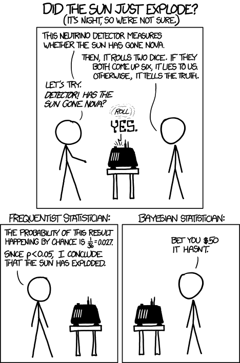
I meant this as a jab at the kind of shoddy misapplications of statistics I keep running into in things like cancer screening (which is an emotionally wrenching subject full of poorly-applied probability) and political forecasting. I wasn’t intending to characterize the merits of the two sides of what turns out to be a much more involved and ongoing academic debate than I realized. A sincere thank you for the gentle corrections; I’ve taken them to heart, and you can be confident I will avoid such mischaracterizations in the future!

Another discussion can be found here.

What problems is it used for?

There are many cases in which we care not only about our estimates, but also how confident we are in those estimates. Some examples:

• Finding a wreckage: In 2009, a passenger plane crashed over the atlantic ocean. For two years, investigators had not been able to find the wreckage of the plane. In the third year, after bringing in Bayesian analysis, the wreckage was found after one week of undersea search (Stone et al 2014)!

• Routing: Understanding the time it takes for vehicles to get from point A to point B. This could be ambulance routing for instance. Knowing the uncertainty in the estimates is important when planning (Woodard et al 2017).

• Microcredit: Is microcredit actually helping? Knowing the extent of the microcredit effect and our certainty about it may be used to make decisions such as making an investment (Meager et al 2019).

These are just some of the applications. There are many more. Hopefully you are convinced that we are doing something useful. Let’s move on to the actual techniques.

How Bayesian inference works—a quick overview

The first step in any inference job is defining a model. We might for example model heights in a population of, say, penguins, as being generated by a Gaussian distribution with mean \(\mu\) and variance \(\sigma^2\).

Our goal is then to find a probability distribution over the parameters in our model, \(\mu\) and \(\sigma^2\), given the data that we have collected. This distribution, also called the posterior, is given by

\[P(\theta \vert y_{1:n}) = \frac{P(y_{1:n} \vert \theta) P(\theta)}{P(y_{1:n})},\]

where \(y_{1:n}\) represents the dataset containing \(n\) observations and \(\theta\) represents the parameters. This identity is known as Bayes’ Theorem.

In words, the posterior is given by a product of the likelihood \(P(y_{1:n} \vert\theta)\) and the prior \(P(\theta)\), normalized by the evidence \(P(y_{1:n})\).

Sketch of the Bayesian update. The posterior (blue) is obtained after multiplying the prior (red) with the likelihood (black). In a sequential estimation procedure, the new prior is the posterior obtained in the previous step.

The likelihood \(P(y_{1:n} \vert\theta)\) is often seen as a function of \(\theta\), and tells us how likely it is to have observed our data given a specific setting of the parameters. The prior \(P(\theta)\) encapsulates beliefs we have about the parameters before observing any data. We update our beliefs about the parameter distribution after observing data according to Bayes’ rule.

After obtaining the posterior distribution, we would like to report a summary of it. We usually do this by providing a point estimate and an uncertainty surrounding the estimate. A point estimate may for example be given by the posterior mean or mode, and uncertainty by the posterior (co)variances.

In summary, there are three major steps involved in doing Bayesian inference:

1. Choose a model i.e. choose a prior and likelihood.
2. Compute the posterior.
3. Report a summary: point estimate and uncertainty, e.g. posterior means and (co)variances.

In this post, we will not be concerned with the first step, and instead focus on the last two steps: computing the posterior and reporting a summary. This means that we assume someone has already done the modeling for us and has asked us to report back something useful.

The problem, a solution, and a faster solution

Computing the posterior and reporting summaries is generally not a simple task. To see why, consider again the equation we use to compute the posterior:

\[P(\theta \vert y_{1:n}) = \frac{P(y_{1:n} \vert \theta) P(\theta)}{P(y_{1:n})}.\]

One issue is that typically, there is no nice closed-form solution for this expression. Usually, we can’t solve it analytically or find a standard easy-to-use distribution. Another issue is that to find a point estimate such as the mean, or to compute the normalizing constant \(P(y_{1:n})\), we need to integrate over a high-dimensional space. This is a fundamentally difficult problem, and is also known as the curse of dimensionality. The problem is exacerbated by the large and high-dimensional datasets we have these days. (Why does calculating \(P(y_{1:n})\) involve integration? Because it is a marginal obtained by integrating out the parameters: \(P(y_{1:n}) = \int P(y_{1:n}, \theta) d\theta\).)

This is where approximate Bayesian inference comes in. The gold standard in this area has been Markov Chain Monte Carlo (MCMC). It is extremely widely used and has been called one of the top 10 most influential algorithms of the 20th century. MCMC is eventually accurate, but it is slow. In many applications, we simply don’t have the time to wait until the computation is finished.

A faster method is called Variational Inference (VI). In this post, we’ll take a deeper dive into how this works.

Variational Inference and the Mean Field Variational Bayes (MFVB) framework

The main idea in VI is that instead of trying to find the real posterior distribution \(p(\cdot \vert y)\), we approximate it with a distribution \(q\). Of course, not every distribution would be useful as an approximation. For some distributions, measures that we’d like to report, like the mean and variance, can’t be found. We therefore restrict our search to \(Q\), the space of distributions that have certain “nice” properties. We’ll discuss later what “nice” means exactly. In this space, we search for a distribution \(q^*\) that minimizes a certain measure of dissimilarity to \(p\). Mathematically:

\[q^* = argmin_{q\in Q} f(q(\cdot), p(\cdot \vert y)),\]

where \(f\) is some measure of dissimilarity.

KL-divergence

There are many measures of dissimilarity to choose from, but one is particularly useful: the Kullback-Leibler divergence, or KL-divergence.

KL-divergence is a concept from Information Theory. For distributions \(p\) and \(q\), the KL-divergence is given by

\[KL(p\ \vert\vert\ q) = \int p(x)\ln \frac{p(x)}{q(x)}dx.\]

Intuitively, there are three cases of importance:

• If \(p\) is high and \(q\) is high, then we are happy i.e. low KL-divergence.
• If \(p\) is high and \(q\) is low then we pay a price i.e. high KL-divergence.
• If \(p\) is low then we don’t care i.e. also low KL-divergence, regardless of \(q\).

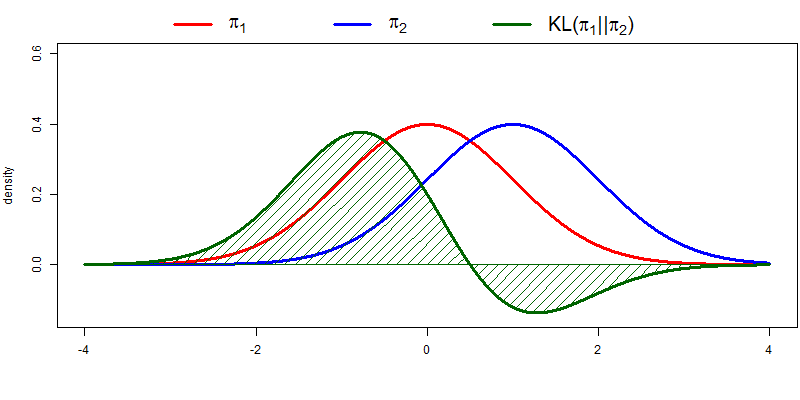
The following figure illustrates KL-divergence for two normal distributions \(\pi_1\) and \(\pi_2\). A couple of things to note: divergence is indeed high when \(p\) is high and \(q\) is low; divergence is 0 when \(p = q\); and the complete KL-divergence is given by the area under the green curve.

KL divergence between two normal distributions. In this example \(\pi_1\) is a standard normal distribution and \(\pi_2\) is a normal distribution with a mean of 1 and a variance of 1. The value of the KL divergence is equal to the area under the curve of the function. (Source)

Loosely speaking, KL-divergence can be interpreted as the amount of information that is lost when \(q\) is used to approximate \(p\). I won’t be going much deeper into it, but it has a couple of properties that are interesting for our purposes. The KL-divergence is:

• Not symmetric: \(KL(p\ \vert\vert\ q) \neq KL(q\ \vert\vert\ p)\) in general. It can therefore not be interpreted as a distance measure, which is required to be symmetric.

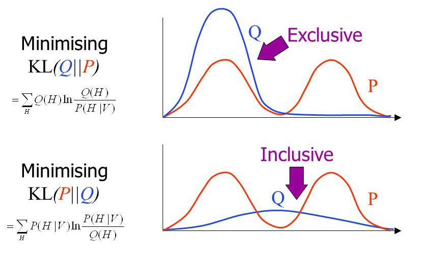
  We will be using the KL-divergence \(KL(q\ \vert\vert\ p)\). It is possible to use the reverse KL-divergence \(KL(p\ \vert\vert\ q)\) as well. Let’s examine the differences.

  In practical applications, the true posterior will often be a multimodal distribution. Minimizing KL-divergence leads to mode-seeking behavior, which means that most probability mass of the approximating distribution \(q\) is centered around a mode of \(p\). Minimizing reverse KL-divergence leads to mean-seeking behavior, which means that \(q\) would average across all of the modes. This would typically lead to poor predictive performance, since the average of two good parameter values is usually not a good parameter value itself. This is illustrated in the following figure.

Minimizing \(KL(q\ \vert\vert\ p)\) versus \(KL(p\ \vert\vert\ q)\). The first (exclusive) leads to mode-seeking behavior, while the latter (inclusive) leads to mean-seeking behavior. (Source Tim Vieira's blog, figure by John Winn.)

For a more in-depth discussion, see Tim Vieira’s blog post KL-divergence as an objective function.

• Always \(\geq 0\), with equality only when \(p = q\). Lower KL-divergence thus implies higher similarity.

Most useful for us though is the following. We are optimizing \(q\) to be as close as possible to the real distribution \(p\), but we don’t actually know \(p\). How do we find a distribution close to \(p\) if we don’t even know what \(p\) itself is? It turns out that we can solve this problem by doing some algebraic manipulation. This is huge. Let’s derive the necessary expression:

\[\begin{align} KL(q\ \vert\vert\ p(\cdot \vert y)) :=& \int q(\theta)\log \frac{q(\theta)}{p(\theta \vert y)}d\theta \\ =& \int q(\theta)\log \frac{q(\theta)p(y)}{p(\theta , y)} d\theta \\ =&\ \log p(y)\int q(\theta)d\theta - \int q(\theta)\log \frac{p(y, \theta)}{q(\theta)} d\theta.\\ =&\ \log p(y) - \int q(\theta)\log \frac{p(y \vert \theta) p(\theta)}{q(\theta)} d\theta. \end{align}\]

Here we use Bayes’ theorem to substite out \(p(\theta\vert y)\) in the second line. Then, we use the property of logarithms \(\log(ab) = \log(a) + \log(b)\), together with the fact that \(p(y)\) doesn’t depend on \(\theta\), and that \(\int q(\theta) d\theta = 1\) since \(q(\theta)\) is a probability distribution over \(\theta\), to arrive at the result. Phew, that was a whole mouthful.

Since \(p(y)\) is fixed, we only need to consider the second term, which has a name: the Evidence Lower Bound (ELBO). We can see from the last equation why it is called this way. \(KL(q\ \vert\vert\ p) \geq 0\) implies \(\log p(y) \geq \text{ ELBO}\). It is thus a lower bound on the log evidence \(\log p(y)\).

To minimize KL-divergence, we thus need to maximize the ELBO. The ELBO depends on \(p\) only through the likelihood and prior, which we already know! This is something we can actually compute without having to know the real distribution!

Mean Field Variational Bayes (MVFB)

I promised to tell you what kinds of distributions we think of as “nice”. Firstly, we want to be able to report a mean and a variance, so these must exist. We then make the MFVB assumption, also known as Mean-Field Approximation. The approximation is a simplifying assumption for our distribution \(q\), which factorizes the distribution into independent parts:

\[q(\theta) = \prod_i q_i(\theta_i).\]

From a statistical physics point of view, “mean-field” refers to the relaxation of a difficult optimization problem to a simpler one which ignores second-order effects. The optimization problem becomes easier to solve.

Note that this is not a modeling assumption. We are not saying that the parameters in our model are independent, which would limit us only to uninteresting models. We are only saying that the parameters are independent in our approximation of the posterior.

We often also assume a distribution from the exponential family, since these have nice properties that make life easier.

Now that we have defined a space and metric to optimize over, we have a clearly defined optimization problem. At this point, we can use any optimization technique we’d like to find \(q^*\). Typically, coordinate gradient descent is used.

When can we trust our method

Since Variational Inference is an approximate method, we’d like to know how accurate the approximation actually is. In other words, when we can trust it. If we schedule an ambulance based on the prediction that it will take 10 minutes to arrive, we have to be damn sure that our confidence in the prediction is justified.

One way to check whether the method works is to consider a simple example that we know the correct answer to. We can then see how well MFVB approximates that answer. To do this, we consider the (rather randomly chosen) problem of estimating midge wing length.

Estimating midge wing length

Note that understanding all the details in this example is not required for an understanding of the big picture.

Midge is a term used to refer to many species of small flies. Before we can compute a posterior, we need a model. As before, we assume that we are given a model, which is determined by a likelihood and a prior. We only need to worry about computing a posterior and reporting back a summary. The model given to us is the following.

Assume midge wing length is normally distributed with unknown mean \(\mu\) and unknown precision \(\tau\). (We use precision, the inverse of variance, because it’s mathematically more convenient.) Let \(y\) be the midge wing length. We care about finding the posterior

\[p(\mu, \tau \vert y_{1:N}) \propto p(y_{1:N} \vert \mu, \tau) p(\mu, \tau).\]

The likelihood is then given by

\[p(y_{1:N} \vert \mu, \tau) = \prod_i \mathcal{N}(y_i \vert \mu, \tau^{-1}),\]

where \(\mathcal{N}(\cdot)\) denotes the normal distribution.

The conjugate prior for a Gaussian with unknown mean and variance is a Gaussian-Gamma distribution given by

\[p(\mu, \tau) = \mathcal{N}(\mu \vert \mu_0, (\beta\tau)^{-1})Gamma(\tau \vert a, b),\]

where \(Gamma\) is the Gamma distribution and \(\mu_0, \beta, a, b\) are hyperparameters.

To start solving the problem, we first use the mean-field assumption resulting in the factorization:

\[q^*(\mu, \tau) = q_\mu^*(\mu)q_\tau^*(\tau) = argmin_{q\in Q_{MFVB}} KL(q(\cdot)\ \vert\vert\ p(\cdot \vert y)).\]

The factors \(q_\mu^*(\mu)\) and \(q_\tau^*(\tau)\) can be derived [Bishop 2006, Sec. 10.1.3]:

\[\begin{align} q_\mu^*(\mu) &= \mathcal{N}(\mu \vert m_\mu, \rho_\mu^2)\\ q_\tau^*(\tau) &= Gamma(\tau \vert a_\tau, b_\tau), \end{align}\]

where “variational parameters” \(m_\mu, \rho_\mu^2, a_\tau, \text{ and } b_\tau\) determine the approximating distribution.

We then iterate. First, we make an initial guess for the variational parameters. Then, we cycle through each factor. We find the approximating distribution of \(\mu\) given the distribution of \(\tau\) in one step and the approximating distribution of \(\tau\) given the distribution of \(\mu\) in another step:

\[\begin{align} (m_\mu, \rho_\mu^2) &= f(a_\tau, b_\tau)\\ (a_\tau, b_\tau) &= g(m_\mu, \rho_\mu^2). \end{align}\]

We repeat this procedure until convergence.

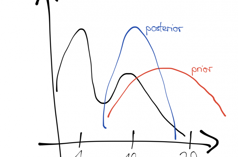
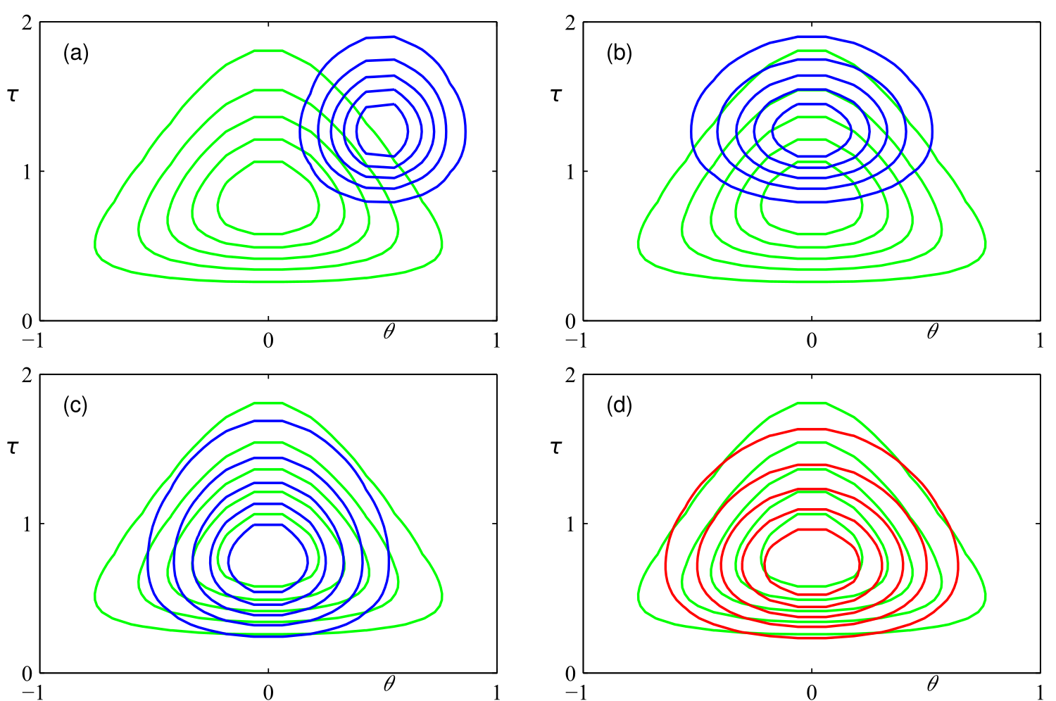
The following figure shows how our approximation (blue) of the real posterior (green) gets more and more accurate by applying coordinate descent, resulting in quite a good approximation (red).

The process of variational approximation to the Gaussian-gamma distribution. Our approximation (blue) of the real posterior (green) gets more and more accurate by applying coordinate descent, resulting in quite a good approximation (red) (Source: PRML, Bishop 2006)

Variance underestimation

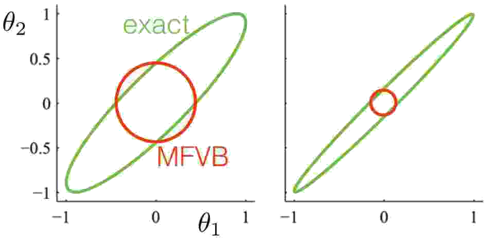
One of the major problems that shows up is that the variational distribution often underestimates the variance of the real posterior. This is a result of minimizing the KL-divergence, which encourages a small value of the approximating distribution when the true distribution has a small value. This is showcased in the next figure, where MFVB is used to fit a multivariate Gaussian. The mean is correctly captured by the approximation, but the variance is severely underestimated. This gets progressively worse as the correlation between the two variables increases.

The MFVB approximation of the true distribution, a multivariate Gaussian, severely underestimates the true variance. This gets worse as the correlation increases (Source: Turner, Sahani 2010).

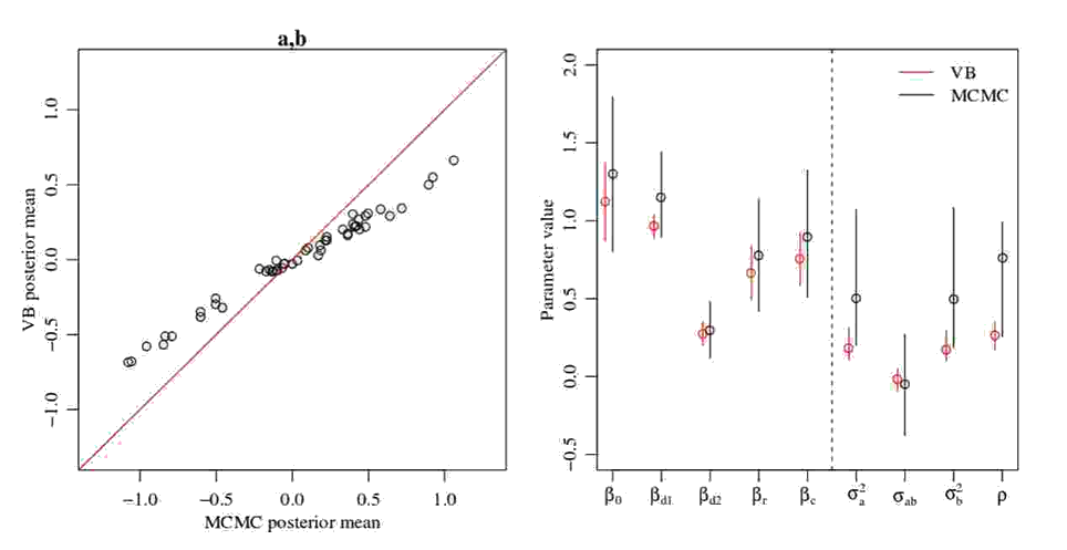
Another way to test the validity of our approximations is to compare them to the answers of a method that we know works: MCMC. We can use this for more complex problems for which we cannot find an analytical solution. One real-life application deals with microcredit.

Microcredit is an initiative that helps impoverished people become self-employed or start a business by giving them extremely small loans. Of course, we’d like to know if this approach actually has a positive effect, how large this effect is, and how certain we are of that.

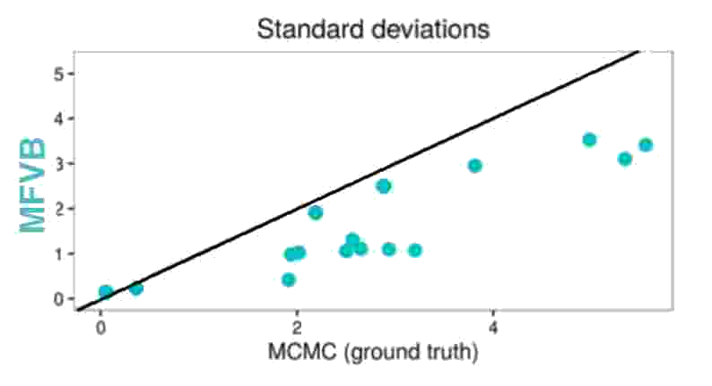
The next figure shows once more that MFVB estimates of microcredit effect variance indeed underestimate the true variance.

Microcredit effect variance estimates given by MCMC versus MFVB. MFVB underestimates variance (Source: Giordano, Broderick, Jordan 2016).

Mean estimates

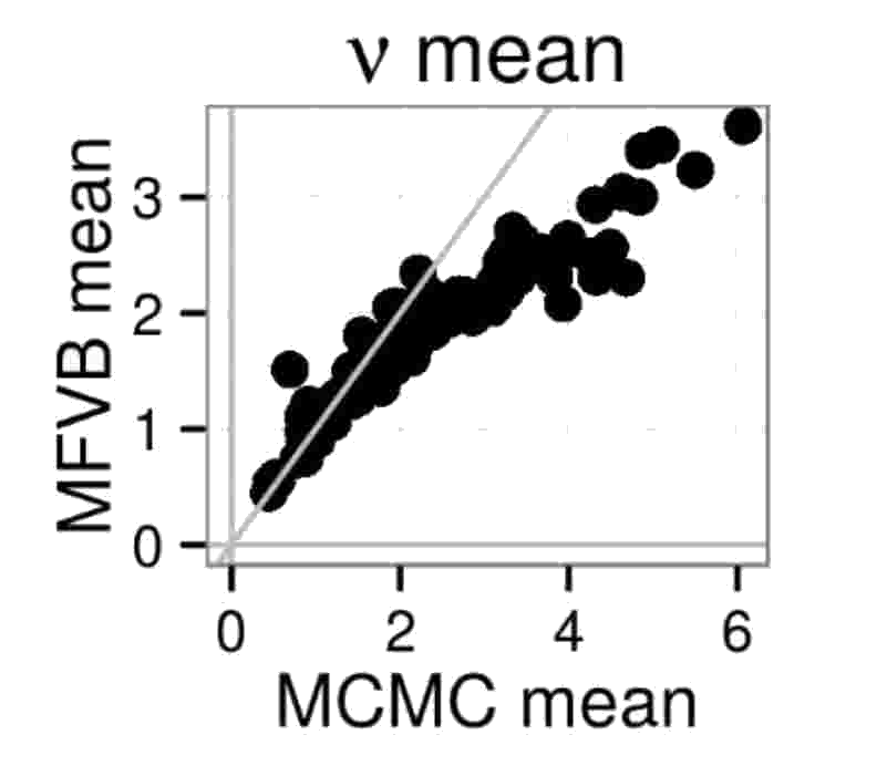
MFVB not always getting the variance right begs another question: Can estimates of the mean be incorrect too? The answer is yes, as demonstrated by the following two figures. In the first figure, MFVB estimates for the mean of a parameter \(\nu\) disagree with MCMC estimates. The same happens in the second figure, where some MFVB estimates are even outside the 95% credible interval obtained by MCMC.

MFVB estimates for the mean of a parameter disagree with MCMC estimate (Source: Giordano, Broderick, Jordan 2015).

MFVB estimates disagree with MCMC estimates (Source: Fosdick 2013).

What can we do?

We’ve seen that MFVB doesn’t always produce accurate approximations. What do we do then? Some major lines of research to alleviate this problem are:

• Reliable diagnostics: Fast procedures that tell us after the fact if the approximation is good. One way to achieve this might be to find a fast way to find the KL-divergence of our approximation, since we know it is bounded below by 0. Usually, we only have access to the ELBO, of which we don’t have such a bound.

• Richer “nice” set: In the MFVB framework, we only consider optimizing over a set of functions that factorize. Considering a richer set of functions might help. It turns out though that having a richer nice set doesn’t necessarily yield better approximations. We’d have to make other assumptions that complicate the problem as well.

• Alternative divergences: Minimizing other divergences than the KL-divergence might help, but has similar difficulties as the above point.

• Data compression: Before using an inference algorithm, we can consider doing a preprocessing step in which the data is compressed. We would like to have theoretical guarantees on the quality of our inference methods on this compressed dataset.

Until we have a foolproof way to test for the reliability of the estimates obtained by MFVB, it is important to be wary of the results obtained, as they may not always be correct.

Summary

We’ve discussed how Bayesian Variational Inference works. By framing the problem as an optimization problem, we can find results much faster compared to the classic MCMC algorithm. This comes at a price: we don’t always know when our approximation is accurate. This is still very much an open problem that researchers are working on.

Related Publications

If you would like to read further, here are some related publications:

• Bishop. Pattern Recognition and Machine Learning, Ch 10. 2006.
• Blei, Kucukelbir, McAuliffe. Variational inference: A review for statisticians, JASA2016.
• MacKay. Information Theory, Inference, and Learning Algorithms, Ch 33. 2003.
• Murphy. Machine Learning: A Probabilistic Perspective, Ch 21. 2012.
• Ormerod, Wand. Explaining Variational Approximations. Amer Stat 2010.
• Turner, Sahani. Two problems with variational expectation maximisation for time-series models. In Bayesian Time Series Models, 2011.
• Wainwright, Jordan. Graphical models, exponential families, and variational inference. Foundations and Trends in Machine Learning, 2008.

More Experiments:

• RJ Giordano, T Broderick, and MI Jordan. Linear response methods for accurate covariance estimates from mean field variational Bayes. NIPS 2015.
• RJ Giordano, T Broderick, R Meager, J Huggins, and MI Jordan. Fast robustness quantification with variational Bayes. ICML Data4Good Workshop 2016.
• RJ Giordano, T Broderick, and MI Jordan. Covariances, robustness, and variational Bayes, 2017. Under review. ArXiv:1709.02536.

Thanks for reading! Any thoughts? Leave them in the comments below!

If you like this post and would like to get updates on future blog posts, you can fill out your email here:

Name Email